Neurons in the early visual system, consisting of the retina, lateral geniculate nucleus (LGN), and primary visual cortex (V1), respond to light stimuli in restricted regions of the visual field called their receptive fields (RFs). The spatial and temporal structure of the RFs among the neurons in the visual system varies, but they usually consist of two parts; one part that depolarize the cell under illumination and one part that hyperpolarize the cell when illuminated. A typical RF structure is the so-called center-surround RF, consisting of a central disk (center) and a concentric ring (surround), each responding oppositely to light. For example, illumination of the center might increase the firing of a neuron, whereas light in the surround would decrease the firing of that neuron.

Estimating firing rates

The firing rate of a neuron evoked by a stimulus \(s(\mathbf{r},t-\tau) \) can be estimated using a linear kernel as

\( r(t) = r_0 + \displaystyle \int \int D(\mathbf{r},\tau) s(\mathbf{r},t-\tau) d\tau d\mathbf{r} \),

where \( r_0\) is the mean firing rate and \( D(\mathbf{r},\tau) \) is a weighting factor that determines how strongly, and with what sign, the value of the stimulus at point \( \mathbf{r} = (x,y) \) and at time \( t-\tau\) affects the firing rate at time \( t \). For cells in the visual system, the kernel \( D(\mathbf{r},\tau) \) defines the time-space RF of a neuron.

An intuitive interpretation of the linear estimate of the equation above can be obtained by performing maximum stimulus analysis[1], where the result is that the stimulus producing the maximum response (at fixed stimulus energy) is proportional to the optimal kernel \( D(\mathrm{r},\tau) \). This means that the integral above measures the overlap between the actual stimulus and the most effective stimulus. A large overlap between these two increases the value of the integral resulting in a large firing rate \( r(t)\), while mismatches give lower predictions for the firing rate.

Spatial receptive fields

Some neurons have separable space-time RF, meaning that the RF can be written as product of two functions; one that describe the spatial structure of the RF and the other the temporal RF:

\( D(\mathbf{r},\tau) = D_s(\mathbf{r}) D_t(\tau) \).

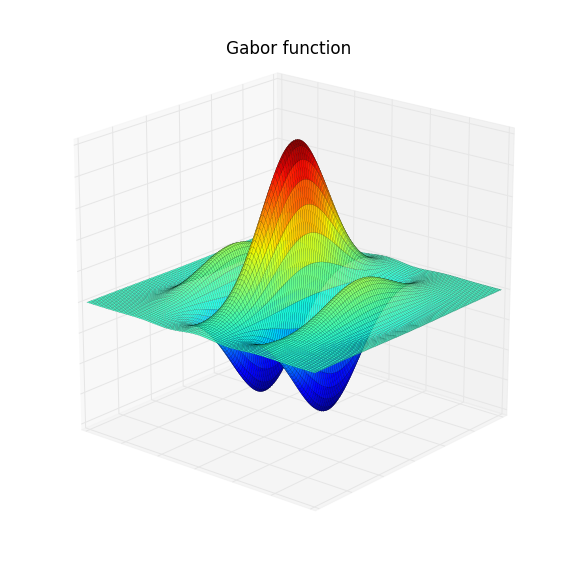
In these neurons the spatial structure of the RF does not change over time except by an overall multiplication factor. A popular mathematical approximation of the spatial RF of simple cell is the Gabor function, which is a product of a Gaussian function and a sinusoidal function:

\( D_s(x,y) = \frac{1}{2\pi \sigma_x \sigma_y} \mathrm{exp}\left(-\frac{x^2}{2\sigma_x^2} - \frac{y^2}{2\sigma_y^2}\right)\cos(kx - \phi) \).

The parameters \( \sigma_x \) and \( \sigma_y \) determine the extent in the \(x \) and \( y \) direction respectively, \(k\) is the preferred spatial frequency and \( \phi \) is the preferred spatial phase. In the figure below the Gabor function is shown for some given parameters. The red regions corresponds to the ON-part of the RF and the blue regions are the OFF-part of the RF.

Receptive fields in Neuronify

In Neuronify several types of RFs can be chosen. These are defined as 2D matrices with user-defined dimensions that can be adjusted in the option menu of Retina objects. The simplest RF-types in Neuronify are the one where half of the matrix is set to +1 (white) and the other half -1 (black), representing the ON and OFF regions of the spatial RF (see figure below).

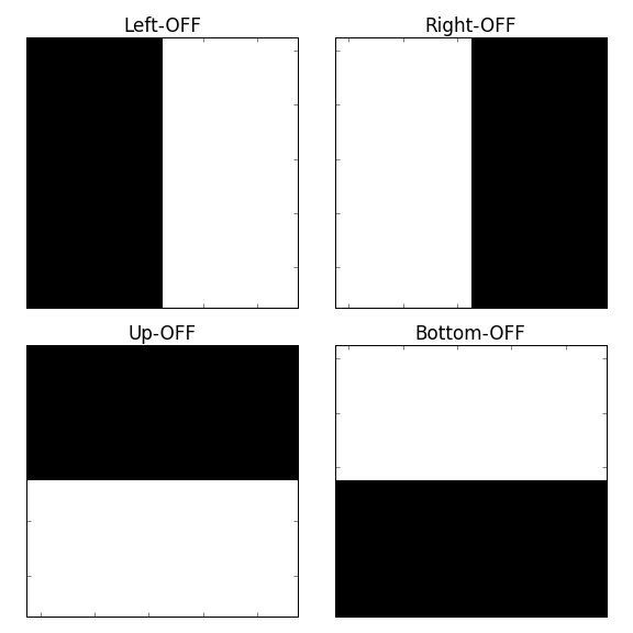
When the frame seen by the camera consists of a dark area and a light area that overlap with the negative and positive part of the matrix, respectively, we will get high activity. The opposite, dark on positive part and light on negative part, will silence the cell.

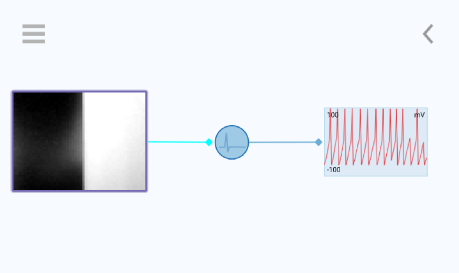
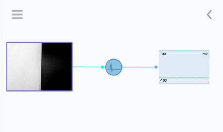
Here you see how a cell with left-OFF RF will respond to different stimulus:

References

[1] Peter Dayan and L. F. Abbott. 2005. Theoretical Neuroscience: Computational and Mathematical Modeling of Neural Systems. The MIT Press.